Assessing Child Density
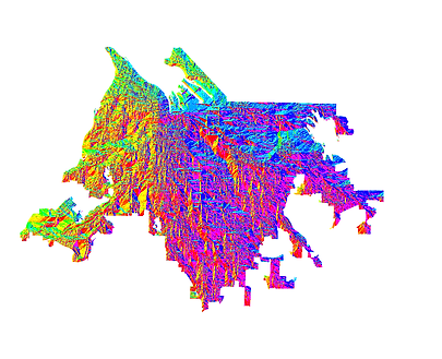
Using the child density point data created to analyze the need for toxic remediation in Pierce County, a hot spot analysis was performed to determine areas of high and low child density based on z-score (the distance of a value from the mean) at the blocks enumeration level for the entire Tacoma/Pierce County Urban Metro Area (Fig. 1). Areas symbolized red indicate a high child density and areas symbolized blue indicate a low child density.
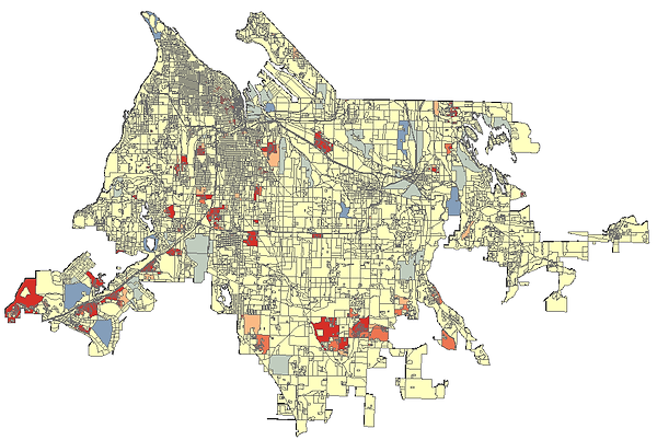
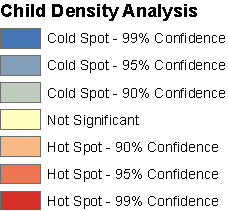
Fig. 1
This analysis is only interested in areas with a high child density, so within the attribute table of the hot spot analysis, the blocks with the highest child density z-score that also held a p-value (the chance that the z-score is statistically random) below 10% were isolated and exported to create a new polygon feature class (Fig. 2).

Fig.2
This analysis is particularly interested in identifying larger areas where there are concentrations of young children. Therefore it is necessary to identify clusters of several blocks. To do that the high child density polygons from Fig. 2 were aggregated to points with an aggregation distance of 2000-feet (points within that distance from each other will be combined) to produce a new polygonal feature class containing the aggregated point data (Fig. 3).
Because this analysis is particularly interested in larger areas with high child density, the largest polygon (by area) was selected from the feature class depicted in Fig. 3 and converted to a point which will serve as the starting point for a cost path analysis (Fig. 4).
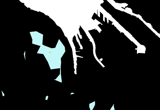
Fig. 4

Fig. 3
Fig. 5
Finding Large Parks Nearest the Largest Area with the Highest Child Density

The purpose of the cost path analysis is to define paths between the largest area with a high child density and large parks in the Tacoma/Pierce County Urban Metro Area.
A Pierce County parks polygonal feature class was added, from which parks larger than 50-acres were isolated and exported to create a new feature class containing only large parks (Fig. 5).

The large parks depicted in Fig. 5 serve as the destinations for the cost path analysis. While it would be possible to run the analysis using the point of child density (Fig. 4) as the origin and the centroid of each large park as the destination, this analysis is less concerned with distance to the center of any particular park and more concerned with distance to edge of a given park since, upon arrival, children have a multitude of choices about where to go and what to do.
To determine the distance from the point of child density to the edge of large parks the 'Generate Near Table' tool was used where 5-miles was determined to be the search radius -- the tool will identify and plot at point at the edge of parks within a 5-mile radius of the origin (Fig. 6).
Fig. 5
Fig. 6
Creating the Cost Surface
The cost surface for this analysis will consider slope of terrain, distance from the point of highest child density (Fig. 4), and the classification of streets along which travel will occur. In order to create a functional dataset, the slope, distance, and streets need to be converted to raster form and reclassified to allow for calculation when creating the cost path.
The first step in this process was creating the slope layer for teh Tacoma/Pierce County Metro Area (Fig. 7), then reclassifying it so that a range of slope values were given a numerical classification (1-10). The output of this operation can be seen in Fig. 8.


Fig. 7
Fig. 8
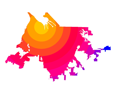

Fig. 9
Fig. 9
Fig. 10
To determine distance from the point of highest child density, the Euclidian Distance tool was used. The result of he operation can be seen in Fig. 9. The data was then reclassified into 10 classes so that different ranges of distance values were given a numerical classification. The output of this operation can be seen in Fig. 10


Fig. 11
Fig. 11
Fig. 12
Line data representing streets for Pierce County were clipped to the Tacoma/Pierce County Metro Area (Fig. 11), and given a classification (1-9) within the attribute table with streets with slower speed limits given lower values than streets with higher speed limits. After these calculations were performed, the streets data was converted to a raster based on the previously discussed classification. A portion of the output of this operation is visible in Fig. 12. A reclassification operation was performed in order to give areas with no data (i.e. off road areas) a classification of 10, with the goal of making off road travel prohibitive for the cost analysis.

A raster calculation was performed using the reclassified slope, distance, and streets rasters where each was given a weight relative to their impact on the travel path. Roads classification was given 50% of the total weight,slope was given 30%, and distance was given 20%. The output of this operation was a single raster containing the calculated value (Fig. 13)
Fig. 13
The cost distance tool was utilized to calculate the cost of traveling over each individual cell in the raster that was created in Fig. 13. The output of this operation was two rasters: 1) a distance raster containing the accumulative cost distance over a cost surface to the point of highest child density (Fig. 14), and 2) a backlink raster which can be used to identify the least costly direction of travel from one cell in the cost surface to another (Fig. 15). The distance and backlink rasters are used as inputs for a cost path analysis.

Determining Cost Paths
The purpose of the cost path analysis is to define the least costly paths between the point of highest child density and large parks in the Tacoma/Pierce County Metro Area -- paths with a low aggregate score for slope, distance, and road classification. To determine the least costly paths, the Cost Path tool was utilized where the distance and backlink rasters (Fig. 14-15) were used as inputs for the tool to calculate cost paths. The calculated paths can be seen in Fig. 16. Fig. 17 shows the calculated path from the point of highest child density to the nearest large park and Fig. 18 shows the calculated path with streets and street names.
Fig. 14
Fig. 14
Fig. 15

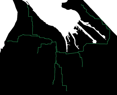
Fig. 16

Fig. 17
Fig. 18
